Introduction

This is a mini-project that models and simulates of lane change maneuvers of autonomous vehicles. Here we construct a bicycle model for each vehicle and solve the dynamical system based on state-space equations. Using LQR linear controller, we construct a closed-loop model of the system and simulate the whole process by MATLAB/Simulink. The results can verify our design, to a certain extent.

The lane change strategy can be divided according to the existence of road infrastructure or reference trajectory. Here, we provide a model that could display the maneuver of lane change and express the security based on the simulation. To specify, our model includes four autonomous vehicles, where three cars are driving in the right lane and one is in the left lane. The purpose is that the vehicle in the left lane wants to move to the right while avoiding collisions. Suppose that each vehicle is equipped with sensors (with reasonable errors) and can communicate with its neighboring cars (send necessary information). This maneuver can be considered as an automated process.

The vehicle dynamics are represented by a dynamic bicycle model, and each vehicle is composed of a linear controller (which is LQR controller actually) that regulates its own lateral and longitudinal behavior. In order to ensure safe handling and meet traffic regulations, we use a cooperative driving control scheme that determines the actions of each vehicle.

Model - System Description

In this section, we present the details of the scenario and describe the whole system. At first, let’s consider the real scenario on the road. There are four vehicles on the road, three of them are on the right lane with same speed and another one are on the left lane. Now we want to implement one maneuver of automated merging maneuver, i.e. how to insert a vehicle from the on-ramp in the middle between two pre-selected vehicles of a platoon in the main lane. Specifically, the vehicle on the lane has to merge to the right one, because of high layers like road infrastructure or the emergency, e.g. obstacle avoidance.

Suppose that all vehicles are equipped with sensors used to measure the orientation, position and velocity. Besides, all vehicles have the capacity to communicate with their neighboring vehicles, the important information are longitudinal position and speed.

Notice that, we suppose the width of each lane is 5m, and we take the y coordinate of middle line of the right lane as 0.

System Specifications

Before design the model, we should define the specifications of our system. For each vehicle, we care about its safety margins with surrounding vehicles, the respect for traffic rules and the physical constraints,etc. More precisely, they could be interpreted as:

1. The distance of two neighboring vehicles of the platoon should always maintain larger than a given threshold,

2. The vehicles of the platoon should maintain a constant time gap($t_{gap}$) (a.k.a time-to-collision) between each other;

3. The manoeuvre should only be initiated if the time gap is greater than a given value($t_{gap_m}$),

4. Once the manoeuvre is finished, the vehicles should form a platoon and the velocity of all vehicles should reach $|v_{des} \pm \epsilon |$, where $\epsilon$ is a user-defined metric,

5. The practical velocity bounds of vehicles exist, e.g. $v_{min} \leq v \leq v_{max} $,

6. The control inputs are bounded.

Vehicle Dynamics

For vehicle dynamics, there are a large variety of models. As in the literature of autonomous vehicles, dynamic and kinematic bicycle models are commonly used. In this case, instead of a kinematic model, a dynamic model for lateral vehicle motion must be developed. So we consider a dynamic bicycle model with a linear tire model. The model is assumed linear to avoid computational complexity.

The state vector contains (we take the position of the rear axle of vehicles as the reference of longitudinal and lateral position):

• the longitudinal position of the rear axle $p_{x,r}$
• the lateral position of the rear axle $p_{y,r}$
• the yaw angle $\psi$
• the longitudinal velocity $v_x$
• the lateral velocity at the center of the rear axle $v_y$
• the yaw rate $\omega$

The inputs of command are the longitudinal acceleration $a_x$ and the steering angle $\delta$. The state vector is measured and we model additive measurement noise in all state dimensions, which are $e^m_{x,r}, e^m_{y,r}, e^,{\psi}, e^m{v_x}, e^m_{v_y}, e^m_{\omega}$.

Starting from first-principles, the differential equations of the dynamic bicycle model are defined:

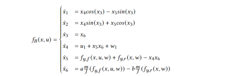
Linearization

The nonlinear model is linearized around a set of operating points using standard point-wise linearization.For linearization purposes in our case, because of the stable equilibrium and the destined velocity of vehicles(we set as 70 km/h), we consider a set point $x_{op} = [0; 0; 0; 70/3.6; 0; 0]$ and do Taylor expansion around the point.

Linear Controller

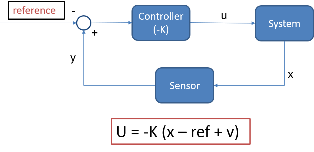
The objective of the linear controller of each vehicle is to regulate its position and velocity in accordance with the behavior of the other vehicles. At the same time, the lane change maneuver should be safety. Once the maneuver is completed, the vehicle platoon should maintain the predefined vehicle speed $v_{des}$.

\($ u = -K\cdot y = -K\cdot(x+v)\)$

We opt for an LQR (Linear Quadratic Regulation) controller since it is a well established design technique that provides practical feedback gains. LQR is an optimal multivariable feedback control approach which minimizes the deviation of the state trajectories of the closed-loop system while requiring minimum controller effort. The behavior of an LQR controller is determined by two parameters: state and control weighting matrices. These two matrices are design parameters and influence the success of the LQR controller synthesis.Now we need to determine the weighting matrices of the cost function.

Supervisory Control

You are able to find more details in the Report PDF.

Simulation

We simulate the whold model by MATLAB/Simulink. At first we construct the control model for each vehicle. Then, connect all vehicles following the dependencies between each other. We construct the global system and realize the communication among the vehicles, using the basic information(longitudinal position and velocity, etc).

The global model and the curves displays could be represented below. The references come from the output of other vehicles, with the errors of sensors. The signal processing and dynamical control are realised separately by models of each vehicle.

Example of leader Vehicle

For the merging vehicle, we need to consider it as a special case. As we have divided the lane change maneuver into two phase, we need to set one logic switching based on the condition $\phi$ we have defined.

Simulation Results

To make a clear implementation of the lane change maneuver and ignore the unnecessary errors($e_\psi^m$ and $e_\omega^m$), we get a complete/dynamic lane change process for our case. Here, circles stand for the position of the vehicles in the right lane, and star stands for the merging vehicle.

Conclusion

We construct the dynamical model of vehicles by classical bicycle model and study one case of real scenario of lane change using a global system based on the vehicle model. To realize the performance of autonomous control, we design a LQR controller and solve the state-space equations, calculate the feedback gain which is used in the simulation. Also, we design a supervisory control to meet the safety requirements during the merging process, using the references and dependencies of the velocity and position information. Finally, we simulate the lane change maneuver by Simulink and verify the correctness of our system.